6 Extremely Useful Excel Tips That Will Turn You Into a Spreadsheet Pro
Google Sheets is a great tool, and plenty of people use it every day. While the basic functions are no doubt useful, they aren’t the only formulas available. You can automate irritating, time-consuming tasks – or discover more utility, by using these formulas.
Let’s expand on what each of these six formulas is, and why they help so much. Starting with…
IMPORTRANGE

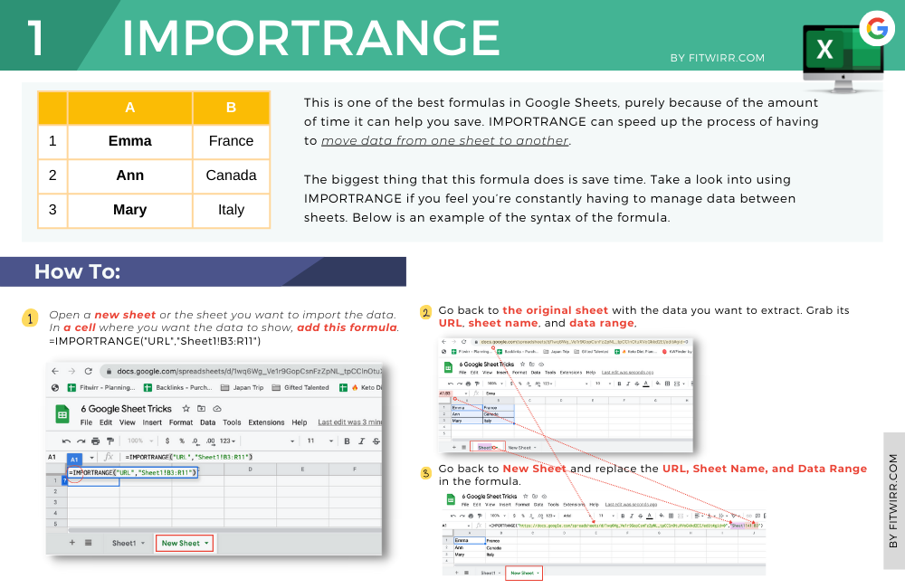
This is one of the best formulas in Google Sheets, purely because of the amount of time it can help you save. IMPORTRANGE can speed up the process of having to move data from one sheet to another.
Rather than having to copy it manually – and waste time, as well as deal with other issues between sheets – IMPORTRANGE skips all of that and does it the easy way.
Not only does it make the transfer of data instant, but Importance also offers even more for those who use it. It’s not complex or hard to use, and being able to link different data sheets together with the knowledge that it will update is very useful.
The biggest thing that this formula does is save time. Take a look into using IMPORTRANGE if you feel you’re constantly having to manage data between sheets. Below is an example of the syntax of the formula.
=IMPORTRANGE(“URL”,”Sheet1!B3:R11″)
IFERROR

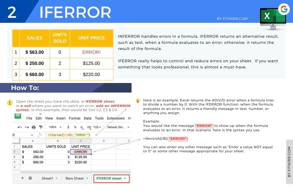
The next killer formula on this list is IFERROR. This is one of the best formulas on this list because it really helps deal with errors, which cause tons of problems across plenty of sheets.
You’ll find yourself running into errors on Google Sheets a lot if you use formulas a ton, or if you have big, complex spreadsheets. Human error is the biggest killer of all, and the more complex your setup is, the more likely that there will be a mistake in there somewhere.
Some formula pointing where it’s not supposed to, a value wrong: it will happen.
IFERROR really helps in these situations (especially if a boss or client is looking at the sheet!) because it helps to control and reduce errors on your sheet. If you want something that looks professional, this is almost a must-have.
Below is the syntax for those interested:
=iferror(E4/D4, 0)
LEN

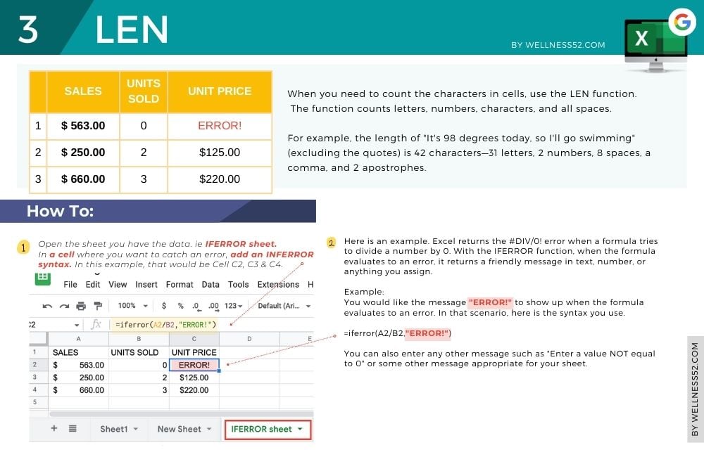
LEN is one of the simpler formulas inside of Google Sheets, but that doesn’t mean that it isn’t useful. In fact, when used correctly, LEN can be a great time saving tool and a simple way to keep track of numbers in your spreadsheet.
The way LEN works is straightforward: it checks a string and reviews the number of characters that it finds there. Those characters are then displayed wherever the formula is placed, so you know how many characters were used in the string you requested.
You can use this for lots of things, but most commonly it’s great if you have certain character limits on something you’re making or producing. LEN is even better if you have different character limits for different kinds of content you’re making.
That way, you’ll always know you’re counting correctly: and if you’re tracking numbers, you want to make sure they come out right. LEN will help with that.
Read the syntax for this useful formula below:
=LEN(E2)
=LEN(“Example Text”)
COUNTIF
The next amazing formula on the list is COUNTIF. This is another great formula that’s useful in both your personal life as well as your professional life. That’s because the function of this formula really saves your time.
What COUNTIF does is checks for a specific value, and then reports back to you and tells you how many times that value appeared. This is great if you’re looking to add up certain amounts of certain items or if you’re trying to track something specific. It also has value in terms of just helping you organize your sheet(s) better.
You can use this in all types of ways and it really has value in a lot of different sheets, so this formula is definitely recommended. Give it a shot!
Check out the syntax of the formula below:
=countif($C$2:$D$21,”Truck”)
=countif($F$2:$G$21,”>75″)
V-LOOKUP
V-LOOKUP is the next irreplaceable formula on this list. V-LOOKUP is useful for retrieving data from interrelated sheets.
You can use this function to retrieve important data and show it on another part in a sheet. This is useful, for example, in the case of needing to mass-check the status of orders on a huge sheet. Another example would be if you had to compare the completion status of a large number of assigned projects between employees.
The more big and complex your sheets, the more useful functions like V-LOOKUP are: they save you manual labor and tons of time. Remember to use $ to declare the range, or errors are inevitable.
If you’re interested in trying V-LOOKUP, review its syntax below:
=VLOOKUP(B3,$H$3:$J$22,2,false)
ARRAYFORMULA
ARRAYFORMULA is a really useful formula in Google Sheets. It can best be described as the quickest, fastest way to perform functions across your entire sheet.
This is one of the best functions when it comes to mass-performing functions. When you have big projects and tons of data, that happens all the time.
ARRAYFORMULA can be used in all kinds of situations. Adding up different cells or ranges of cells is the easiest thing, but other functions can be performed with it.
ARRAYFORMULA is more useful the more numbers and data you have. It’s all about automating and removing manual labor from yourself.
Check out the syntax below to use ARRAYFORMULA:
=ArrayFormula(E2:E+F2:F)
Control Your Data the Convenient Way
All of these formulas are useful in the above ways and more: you just need to not forget the functions. All of these will help save you time, energy, and make your work far easier. These are really some killer formulas!


